This is a multilayer feed forward neural network for text sentiment classification trained on 25,000 movie reviews from the IMDB movie reviews website. The dataset also provides another 25,000 samples which we use after training to test the model. This example project demonstrates text feature representation and deep learning in Rubix ML using a neural network classifier called a Multilayer Perceptron.
Clone the project locally using Composer:
$ composer create-project rubix/sentimentNote: Installation may take longer than usual because of the large dataset.
Make sure you have all the necessary build tools installed such as a C compiler and make tools. For example, on an Ubuntu linux system you can enter the following on the command line to install the necessary dependencies.
sudo apt-get install make gcc gfortran php-dev libopenblas-dev liblapacke-dev re2c build-essentialCompile and install the Tensor 4.1+ extension using PIE:
pie install rubix/tensor_ext:^4.1- PHP 8.3 or above
- Tensor 4.1+ extension for faster training and inference
Our objective is to predict the sentiment (either positive or negative) of a blob of English text using machine learning. We sometimes refer to this type of ML as Natural Language Processing (NLP) because it involves machines making sense of language. The dataset provided to us contains 25,000 training and 25,000 testing samples each consisting of a blob of English text reviewing a movie on the IMDB website. The samples have been labeled positive or negative based on the score (1 - 10) the reviewer gave to the movie. From there, we'll use the IMDB dataset to train a multilayer neural network to predict the sentiment of any English text we show it.
"Story of a man who has unnatural feelings for a pig. Starts out with a opening scene that is a terrific example of absurd comedy. A formal orchestra audience is turned into an insane, violent mob by the crazy chantings of it's singers. Unfortunately it stays absurd the WHOLE time with no general narrative eventually making it just too off putting. ..."
The samples are given to us in individual .txt files and organized by split and label into train and test folders, each of which contains positive and negative subfolders. We'll use PHP's built in glob() function to loop through all the text files in each folder and add their contents to a samples array along with the corresponding positive and negative labels. We'll do this for both the training and testing splits, building a Labeled dataset object for each.
Note: The source code for this example can be found in the train.php file in the project root.
use Rubix\ML\Datasets\Labeled;

$datasets = [];

foreach (['train', 'test'] as $split) {
    $samples = $labels = [];

    foreach (['positive', 'negative'] as $label) {
        foreach (glob("$split/$label/*.txt") as $file) {
            $samples[] = [file_get_contents($file)];
            $labels[] = $label;
        }
    }

    $datasets[] = new Labeled($samples, $labels);
}

[$training, $testing] = $datasets;Neural networks compute a non-linear continuous function and therefore require continuous features as inputs. However, the samples given to us in the IMDB dataset are in raw text format. Therefore, we'll need to convert those text blobs to continuous features before training. We'll do so using the bag-of-words technique which produces long sparse vectors of word counts using a fixed vocabulary. The entire series of transformations necessary to prepare the incoming dataset for the network can be implemented in a transformer Pipeline.
First, we'll convert all characters to lowercase using Text Normalizer so that every word is represented by only a single token. Then, Word Count Vectorizer creates a fixed-length continuous feature vector of word counts from the raw text, Float Type Converter casts those counts to floats, and TF-IDF Transformer applies a sublinear weighting scheme to those counts. Finally, Z Scale Standardizer takes the TF-IDF weighted counts and centers and scales the sample matrix to have 0 mean and unit variance. This last step will help the neural network converge quicker.
The Word Count Vectorizer is a bag-of-words feature extractor that uses a fixed vocabulary and term counts to quantify the words that appear in a document. We elect to limit the size of the vocabulary to 10,240 of the most frequent words that satisfy the criteria of appearing in at least 2 different documents but no more than a certain proportion of documents. In this way, we limit the amount of noise words that enter the training set.
Another common text feature representation are TF-IDF values which take the term frequencies (TF) from the Word Count Vectorizer and weigh them by their inverse document frequencies (IDF). IDFs can be interpreted as the word's importance within the training corpus. Specifically, higher weight is given to words that are more rare. We use the sublinear TF-IDF variant which applies a logarithmic dampening to the term frequencies.
The transformation pipeline from the previous section is defined as a standalone transformer that we'll apply to the datasets before training. We wrap it in a PersistentTransformer with a Filesystem persister so we can save the fitted transformer to disk and reload it later in our validation and prediction scripts. We'll then define the architecture of the neural network and instantiate the Multilayer Perceptron classifier. The network uses two hidden blocks. The first block consists of three Dense layers of 256 neurons each with a SiLU Activation layer after each one (the middle layer has no bias and is followed by a Batch Norm layer). The second block consists of two 128-neuron Dense layers, the first of which has no bias and is followed by a Batch Norm layer, each followed by a Swish activation layer. The network ends with a 2-unit Dense output layer with one neuron per class. We've found that this architecture works fairly well for this problem but feel free to experiment on your own.
use Rubix\ML\Transformers\PersistentTransformer;
use Rubix\ML\Transformers\Pipeline;
use Rubix\ML\Transformers\TextNormalizer;
use Rubix\ML\Transformers\WordCountVectorizer;
use Rubix\ML\Transformers\FloatTypeConverter;
use Rubix\ML\Transformers\TfIdfTransformer;
use Rubix\ML\Transformers\ZScaleStandardizer;
use Rubix\ML\Tokenizers\NGram;
use Rubix\ML\Persisters\Filesystem;

$transformer = new PersistentTransformer(
    base: new Pipeline([
        new TextNormalizer(),
        new WordCountVectorizer(10240, 2, 0.4, new NGram(1, 2)),
        new FloatTypeConverter(),
        new TfIdfTransformer(sublinear: true),
        new ZScaleStandardizer(),
    ]),
    persister: new Filesystem('transformer.rbx', true)
);
use Rubix\ML\PersistentModel;
use Rubix\ML\Classifiers\MultilayerPerceptron;
use Rubix\ML\NeuralNet\Layers\Dense;
use Rubix\ML\NeuralNet\Layers\Activation;
use Rubix\ML\NeuralNet\Layers\Swish;
use Rubix\ML\NeuralNet\Layers\BatchNorm;
use Rubix\ML\NeuralNet\ActivationFunctions\SiLU;
use Rubix\ML\NeuralNet\Optimizers\AdaMax;
use Rubix\ML\NeuralNet\Optimizers\Schedulers\Constant;
use Rubix\ML\Persisters\Filesystem;
$estimator = new PersistentModel(
base: new MultilayerPerceptron(
hiddenLayers: [
new Dense(256),
new Activation(new SiLU()),
new Dense(256, bias: false),
new BatchNorm(),
new Activation(new SiLU()),
new Dense(256),
new Activation(new SiLU()),
new Dense(128, bias: false),
new BatchNorm(),
new Swish(),
new Dense(128),
new Swish(),
new Dense(2),
],
batchSize: 32,
gradientAccumulationSteps: 4,
optimizer: new AdaMax(new Constant(0.0001)),
maxGradientNorm: 1.0,
epochs: 100,
minChange: 1e-5,
evalInterval: 1,
window: 10
),
persister: new Filesystem('model.rbx', true)
);We'll choose a micro-batch size of 32 samples and perform network parameter updates every 4 batches (an effective batch size of 128) using the AdaMax optimizer. AdaMax is based on the Adam algorithm but tends to handle sparse updates better. We hold the learning rate constant at 0.0001 using the Constant scheduler. When setting the learning rate of an optimizer, the important thing to note is that a rate that is too low will cause the network to learn slowly while a rate that is too high will prevent the network from learning at all.
Lastly, we'll wrap the entire estimator in a Persistent Model wrapper so we can save and load it later in our other scripts. The Filesystem persister tells the wrapper to save and load the serialized model data from a path on disk. Setting the history parameter to true tells the persister to keep a history of past saves.
Before we train, we'll set a Screen logger on the estimator so that status messages are printed to the console as training progresses.
use Rubix\ML\Loggers\Screen;

$logger = new Screen();
Remember that the training and testing samples are still raw text at this point, so we need to fit the transformer on the training data and run it over both of the datasets we created before training. First, we call the fit() method on the transformer with the training dataset to learn the vocabulary, weights, and scaling parameters. Then, we call save() to persist the fitted transformer to disk so that we can reload it later in our validation and prediction scripts.
$logger->info('Preprocessing dataset');

$transformer->fit($training);

$transformer->save();
Finally, we use the apply() method to perform the vectorization and normalization on both of the datasets in place, leaving them ready to be fed into the network.
$training->apply($transformer);

$testing->apply($transformer);
Since we're using a separate testing dataset to evaluate the model's generalization during training, we attach it to the estimator as the validation dataset using the setValidationDataset() method. This way, the validation score is calculated on a set of samples that the network has not been trained on at any point.
$estimator->setLogger($logger);

$estimator->setValidationDataset($testing);
Now, you can call the train() method on the learner with the training dataset we instantiated earlier as an argument to kick off the training process.
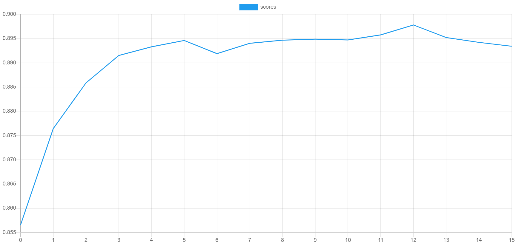
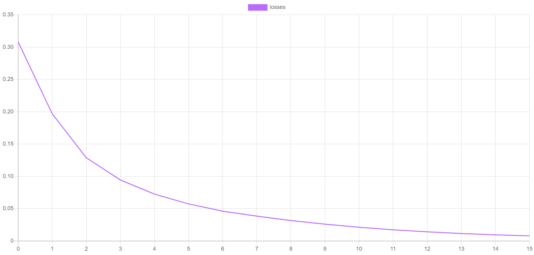
$estimator->train($training);During training, the learner will record the validation score and the training loss for each epoch where they are evaluated. The validation score is calculated using the default F Beta metric on the testing dataset registered as the validation set via setValidationDataset(). Contrariwise, the training loss is the value of the cost function (in this case the Multiclass Cross Entropy loss) calculated over the samples left in the training set. We can visualize the training progress by plotting these metrics. To output the scores and losses you can call the progress() method and pass the resulting iterator to a Writable extractor such as CSV.
Note: The
evalInterval,window, andminChangeparameters on the network control how often scores are evaluated and when training is early-stopped if the validation score stops improving.
use Rubix\ML\Extractors\CSV;

$extractor = new CSV('progress.csv', true);

$extractor->export($estimator->progress());
Here is an example of what the validation score and training loss looks like when they are plotted. The validation score should be getting better with each epoch as the loss decreases. You can generate your own plots by importing the progress.csv file into your plotting application.
Finally, we are prompted to save the model so we can load it later in our validation and prediction scripts. If you answer yes, the save() method serializes the model to disk.
if (strtolower(trim(readline('Save this model? (y|[n]): '))) === 'y') {
    $estimator->save();
}
Now you're ready to run the training script from the command line.
$ php train.phpTo test the generalization performance of the trained network we'll use the testing samples provided to us to generate predictions and then analyze them compared to their ground-truth labels using a cross-validation report. Note that we do not use any training data for cross validation because we want to test the model on samples it has never seen before.
Note: The source code for this example can be found in the validate.php file in the project root.
First, we'll set up a Screen logger so that status messages are printed to the console as the script progresses.
use Rubix\ML\Loggers\Screen;

$logger = new Screen();
We'll then start by importing the testing samples from the test folder like we did with the training samples.
$samples = $labels = [];

foreach (['positive', 'negative'] as $label) {
    foreach (glob("test/$label/*.txt") as $file) {
        $samples[] = [file_get_contents($file)];
        $labels[] = $label;
    }
}
Then, load the samples and labels into a Labeled dataset object using the build() method, randomize the order, and take the first 10,000 rows and put them in a new dataset object.
use Rubix\ML\Datasets\Labeled;

$dataset = Labeled::build($samples, $labels)->randomize()->take(10000);
Next, we'll load the transformer we fitted and saved during training as well as the network we trained earlier. We use the static load() method on the PersistentTransformer and PersistentModel wrappers with the Filesystem persister pointing to the files containing the serialized data. We then call the cleanup() method on the estimator to remove the temporary training state from memory.
use Rubix\ML\PersistentModel;
use Rubix\ML\Transformers\PersistentTransformer;
use Rubix\ML\Persisters\Filesystem;

$transformer = PersistentTransformer::load(new Filesystem('transformer.rbx'));

$estimator = PersistentModel::load(new Filesystem('model.rbx'));

$estimator->cleanup();
Remember that the testing samples are still raw text at this point, so before we can make any predictions we need to run the transformer over the dataset. The apply() method will perform the vectorization and normalization in place, leaving the dataset ready to be fed into the network.
$logger->info('Preprocessing dataset');

$dataset->apply($transformer);
Now we can use the estimator to make predictions on the testing set. The predict() method on the estimator takes a dataset as input and returns an array of predictions.
$logger->info('Making predictions');

$predictions = $estimator->predict($dataset);
The cross-validation report we'll generate is actually a combination of two reports - Multiclass Breakdown and Confusion Matrix. We wrap each report in an Aggregate Report to generate both reports at once. The Multiclass Breakdown will give us detailed information about the performance of the estimator at the class level. The Confusion Matrix will give us an idea as to what labels the estimator is confusing one another for by binning the predictions in a 2 x 2 matrix.
use Rubix\ML\CrossValidation\Reports\AggregateReport;
use Rubix\ML\CrossValidation\Reports\ConfusionMatrix;
use Rubix\ML\CrossValidation\Reports\MulticlassBreakdown;

$report = new AggregateReport([
    new MulticlassBreakdown(),
    new ConfusionMatrix(),
]);
To generate the report, pass in the predictions along with the labels from the testing set to the generate() method on the report. The return value is a report object that can be echoed out to the console.
$results = $report->generate($predictions, $dataset->labels());

echo $results;
We'll also save a copy of the report to a JSON file using the Filesystem persister.
$results->toJSON()->saveTo(new Filesystem('report.json'));Now we can execute the validation script from the command line.
$ php validate.phpTake a look at the report and see how well the model performs. According to the example report below, our model is about 88% accurate.
[
    {
        "overall": {
            "accuracy": 0.8756,
            "accuracy_balanced": 0.8761875711932667,
            "f1_score": 0.8751887769748257,
            "precision": 0.8820119837481977,
            "recall": 0.8761875711932667,
            "specificity": 0.8761875711932667,
            "negative_predictive_value": 0.8820119837481977,
            "false_discovery_rate": 0.11798801625180227,
            "miss_rate": 0.12381242880673332,
            "fall_out": 0.12381242880673332,
            "false_omission_rate": 0.11798801625180227,
            "threat_score": 0.778148276032161,
            "mcc": 0.7581771833363391,
            "informedness": 0.7523751423865335,
            "markedness": 0.7640239674963953,
            "true_positives": 8756,
            "true_negatives": 8756,
            "false_positives": 1244,
            "false_negatives": 1244,
            "cardinality": 10000
        },
        "classes": {
            "positive": {
                "accuracy": 0.8756,
                "accuracy_balanced": 0.8761875711932667,
                "f1_score": 0.8680246127731805,
                "precision": 0.9338050673362246,
                "recall": 0.8109018830525273,
                "specificity": 0.941473259334006,
                "negative_predictive_value": 0.8302189001601709,
                "false_discovery_rate": 0.06619493266377541,
                "miss_rate": 0.1890981169474727,
                "fall_out": 0.05852674066599395,
                "false_omission_rate": 0.16978109983982914,
                "threat_score": 0.7668228678537957,
                "informedness": 0.7523751423865335,
                "markedness": 0.7523751423865335,
                "mcc": 0.7581771833363391,
                "true_positives": 4091,
                "true_negatives": 4665,
                "false_positives": 290,
                "false_negatives": 954,
                "cardinality": 5045,
                "proportion": 0.5045
            },
            "negative": {
                "accuracy": 0.8756,
                "accuracy_balanced": 0.8761875711932667,
                "f1_score": 0.8823529411764707,
                "precision": 0.8302189001601709,
                "recall": 0.941473259334006,
                "specificity": 0.8109018830525273,
                "negative_predictive_value": 0.9338050673362246,
                "false_discovery_rate": 0.16978109983982914,
                "miss_rate": 0.05852674066599395,
                "fall_out": 0.1890981169474727,
                "false_omission_rate": 0.06619493266377541,
                "threat_score": 0.7894736842105263,
                "informedness": 0.7523751423865335,
                "markedness": 0.7523751423865335,
                "mcc": 0.7581771833363391,
                "true_positives": 4665,
                "true_negatives": 4091,
                "false_positives": 954,
                "false_negatives": 290,
                "cardinality": 4955,
                "proportion": 0.4955
            }
        }
    },
    {
        "positive": {
            "positive": 4091,
            "negative": 290
        },
        "negative": {
            "positive": 954,
            "negative": 4665
        }
    }
]
Nice job! Now we're ready to make some predictions on new data.
Now that we're confident with our model, let's build a simple script that takes some text input from the terminal and outputs a sentiment prediction using the estimator we've just trained.
Note: The source code for this example can be found in the predict.php file in the project root.
First, load the transformer and the model from storage using the static load() method on the PersistentTransformer and PersistentModel wrappers and the Filesystem persister pointed to the files containing the serialized data.
use Rubix\ML\PersistentModel;
use Rubix\ML\Transformers\PersistentTransformer;
use Rubix\ML\Persisters\Filesystem;

$transformer = PersistentTransformer::load(new Filesystem('transformer.rbx'));

$estimator = PersistentModel::load(new Filesystem('model.rbx'));
Next, we'll use the built-in PHP function readline() to prompt the user to enter some text that we'll store in a variable.
while (empty($text)) $text = readline("Enter some text to analyze:\n");To make a prediction on the text that was just entered, we wrap it in an Unlabeled dataset and run the transformer over it to convert the raw text into features. Then, we call the predict() method on the estimator and take the first prediction returned. Since we only have one input sample in this case, the ordering is easy!
use Rubix\ML\Datasets\Unlabeled;

$dataset = new Unlabeled([
    [$text],
]);

$dataset->apply($transformer);

$predictions = $estimator->predict($dataset);

$prediction = current($predictions);

echo "The sentiment is: $prediction" . PHP_EOL;
To run the prediction script enter the following on the command line.
php predict.phpOutput
Enter some text to analyze: Rubix ML is really great
The sentiment is: positiveCongratulations on completing the tutorial on text sentiment classification in Rubix ML using a Multilayer Perceptron. We recommend playing around with the network architecture and hyper-parameters on your own to get a feel for how they effect the model. Generally, adding more neurons and layers will improve performance but training may take longer as a result. In addition, a larger vocabulary size may also improve the accuracy at the cost adding additional computation during training and inference.
See DATASET_README. For comments or questions regarding the dataset please contact Andrew Maas.
- Andrew L. Maas, Raymond E. Daly, Peter T. Pham, Dan Huang, Andrew Y. Ng, and Christopher Potts. (2011). Learning Word Vectors for Sentiment Analysis. The 49th Annual Meeting of the Association for Computational Linguistics (ACL 2011).
The code is licensed MIT and the tutorial is licensed CC BY-NC 4.0.